(This post is in a series of posts I started on dev.to)

Describing a linear relationship

In this post I will give an explanation of linear regression, which is a good algorithm to use when the relationship between values is, well, linear. In this post we'll imagine a linear relationship where when the x value (or feature) increases, so does the y value (the label).

With enough labelled data, we can employ linear regression to predict the labels of new data, based on its features.

The equation for linear regression:

Note: This example will only deal with a regression problem with one variable

y = wx + b

• y is the dependent variable - the thing you are trying to predict
• x is the independent variable - the feature - when x changes it causes a change in y
• w is the slope of the line - in our machine learning example it is the weight - x will be multiplied by this value to get the value for y
• b is the bias - it tells us where our line intercepts the y-axis - if b = 0 then line is at the origin of the x and y axes, but this won't always fit our data too well, which is why setting the bias is useful

The algorithm's goal

We want to figure out what values to use for the weight and bias so that the predictions are most accurate when compared to the ground truth.

Remember my violin price predictions example from Machine Learning Log 3: a brief overview of supervised learning? In that article we talked about using different features to predict the change in the price of a violin, where the overall goal was to predict the price of a given violin.

To make it simpler for this article we are going to consider only one variable for our price prediction. We will predict the price of the violin only depending on the age of the violin. We'll pretend that there is a linear relationship such that when the age of the violin goes up the price also goes up (this is vaguely true in the real world).

So as we have it now:

• y = violin price
• x = violin age
• w = ?
• b = ?

We want to find out what values to use for the weight w and the bias b so that we can fit the slope of our line to our data. Then we can use this information to predict the price y from a new feature x.

Visually

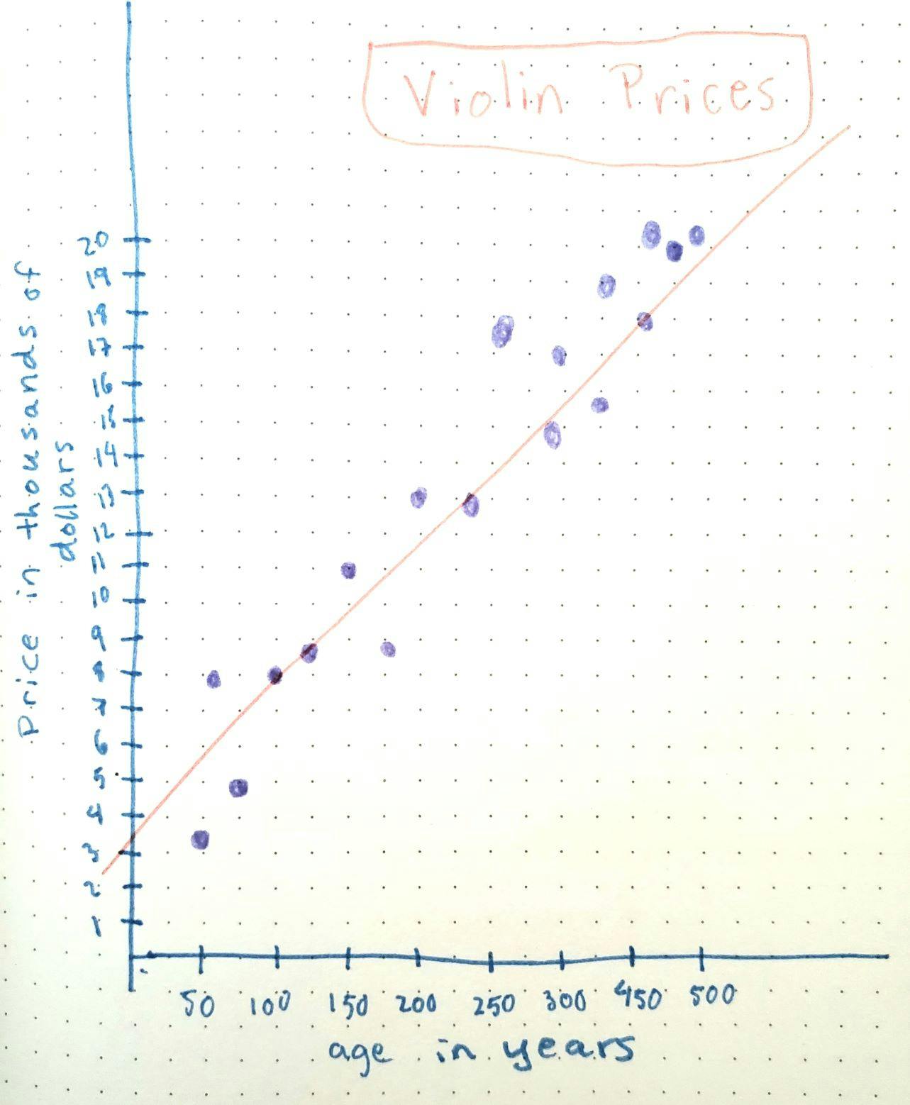
Here's a little graph I drew to represent some possible data points for violins' prices and ages. You can see that when the age goes up so does the price. (This is fictional data, but violins do tend to appreciate in value.)

In code terms:

Let's say we have a 100-year-old violin, that costs, I don't know $8000. We have no idea what to use for w and b yet, so to make our prediction we'll start our weight and bias off at some random number:

Since the weight and bias are started off at random numbers, we're basically taking a stab in the dark guess at this point.

In this case the result of running my little code above was y_prediction = 56.75 which is very wrong (since our ground truth is $8000). This isn't a surprise, since we set our weight and bias to random numbers to begin with. Now that we know how wrong our guess was, we will update the weight and bias to gradually get closer to an accurate prediction that is closer to the real world price of $8000. That is where a cost function and an optimizer come in.

In reality we would be running the predictions with more than just one sample from our dataset of violins. Using just one violin to understand the relationship between age and price won't give us a very accurate predictions, but I presented it that way to simplify the example.

Cost function: seeing how wrong we are

This is where stuff really gets fun! In order to learn from our mistakes we need to have a way to mathematically represent how wrong we are. We do this by comparing the actual price values to the predicted values we got. We find the difference between those values. We use that difference to adjust the weights and bias to fit our values more closely. We rinse and repeat, getting incrementally less wrong, until our predictions are as close as possible to the real world values.

Tune in next week as I explain this process! I'll look at a cost function and describe the process of gradient descent. But I think that's enough for this week. I want to keep these posts fairly short so they can be written and consumed more or less within a Sunday afternoon. 😉

That's all for now, folks!

I am still learning and welcome feedback. As always, if you notice anything extremely wrong in my explanation, or have suggestions on how to explain something better, please let me know in the comments!