


This is the 3rd article in a series on Exploratory Data Analysis, based on my notes on Practical Statistics for Data Science.
For a refresher on what I've discussed so far:
In my last article I discussed estimates of location, such as the mean or median, why they are used, and how they are calculated. In this article we're going to take a look at estimates of variability, which is another facet we can look into when summarizing a feature.
We're going to talk about standard deviation and variance and explain how they differ mathematically.
What is variability?
Variability, also called dispersion, answers the question: Are the data points tightly clustered together or more spread out? There are different ways to measure variability.
"At the heart of statistics lies variability: measuring it, reducing it, distinguishing random from real variability, identifying the various sources of real variability, and making decisions in the presence of it." - from Practical Statistics for Data Science
Deviation
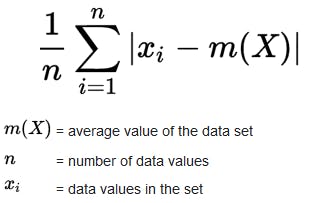
Deviation measures the difference between the estimate of location and the actual observed data. What does this mean? Well if you have a mean of 4 and then the actual values are 3, 4, and 5, the deviations are 1, 0, and -1. The deviations are going to be a set of values where we start with the mean and then subtract each value from it in.
That gives us a list of numbers, which in a large dataset could get quite long. We might not want to look at the deviations for every single value. Remember how the mean was supposed to help us get a quick glance of the central tendency of our data in the first place? Well it seems like we need some sort of average of the deviations to get a quick glance of the typical value for the deviations.
The problem is, we can't just take an average, because the negative deviations will offset the positive ones, and they'll all just sum to 0, which tells us nothing. So instead we'll take the absolute values of the deviations from the mean. This is called the mean absolute deviation and we can compute it like this:
(For a more detailed description of this equation, see Khan academy's article on the subject)
What's absolute value? Absolute value is very simple to compute: take away the minus sign if it is a negative number and if it is a positive number, do nothing. That's the absolute value. In mathematical notation it's depicted between 2 lines. so the absolute value of x looks like |x|.
How does this all tell us about variation? Well it tells us if the data points tend to be clustered around the central value, or spread out from it.
The 2 most common estimates of variability are variance and standard deviation.
What is variance?
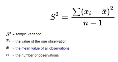
Variance is the average of the squared deviations.
What is Standard deviation?
Standard deviation is the square root of the variance.
Mathematically, it is a little more convenient to work with squared values than with absolute values. Remember, our goal with absolute value was to get rid of the minus sign. (Squaring a value does the same thing, because two negative signs multiplied together give us a positive sign.)
Both variance and standard deviation are pretty sensitive to outliers, especially the standard deviation because it uses a squared value.
- Mean absolute deviation: mean of the absolute values of the deviations from the mean
- Basically you are averaging the deviations themselves but taking the absolute Values
- Aka L1 norm, Manhattan norm
(For a more detailed explanation of how to calculate the standard deviation, see Khan Academy's article on the subject.)
Median absolute deviation from the median:
This value is the median of the absolute values of the deviations from the median. This is a robust estimate of variability, because it is not sensitive to outliers.
Estimates based on Percentiles
Another method of estimating dispersion is looking at the spread of the sorted data. Once our data is sorted, or ranked, it's referred to as order statistics.
- Order statistics: the metrics based in the data values sorted from smallest to biggest
- Aka ranks
We start off with the Range, which is the difference between largest and smallest values in a data set
- In dog food prices example from my EDA part 2 article, it is the difference between 5 and 29
While knowing the minimum and maximum values is important to help identify outliers, knowing the range itself won't tell you much about the dispersion of the data, since this measure is very sensitive to outliers.
To get rid of the outlier problem, we'll just trim the min and max values. Then what we're left with can form the basis for estimates with percentiles.
Percentile: the value where P percent of the values take on this value or less and 100 minus P percent take on this value or more. Example: You want to find the 80th percentile. First, sort the data. Then, start with the smallest value, and go up 80 percent of the way to the largest value.
- Note: The percentile is the same as the quantile, except the quantile is indexed by fractions, so the .8 quantile is the 80th percentile
- The Interquartile range is the range which contains the difference between the 75th percentile and the 25th percentile
- Aka IQR
What's up next?
Next, we'd want to take a look at ways to visualize the data distribution, which I'll cover in a future post.
Further reading
This blog post is based on my notes for Chapter 1 of Practical Statistics for Data Scientists. It contains code examples of data analysis in Python and R.