This post will be an overview of the loss function called mean squared error, as a follow up to last week's discussion of linear regression.

Loss/Error function

Last week we left off our discussion of Linear Regression with recognizing the need for a loss function. After a first look at our prediction, we found that we calculated that a 100 year old violin would cost about $54, instead of the real world value of $800. Clearly, there is some serious work to be done so that our predictions can become more accurate to the real world values. This process is called optimization. And the process begins with a loss function.

Quick review:

Linear regression is based on the equation y = wx + b

We are predicting the y value (the violin's price) based on
the x value - our feature (the violin's age)
multiplied by the weight w
and added to the bias b, which controls where the line intercepts the y-axis
at first w and b are initialized to random weights (in other words, an uninformed guess)

Once we get our first prediction (using the random values for w and b that we chose) we need to find out how wrong it is. Then we can begin the process of updating those weights to produce more accurate values for y.

But first, since so much of machine learning depends on using functions...

In case you forgot what a function is:

I like to think of functions as little factories that take in some numbers, do some operations to them, and then spit out new numbers
the operations are always the same
so, for example, if you put in 2 and get out 4 you will always get out 4 whenever you put in 2
basically a function defines a relationship between an independent variable (x) and a dependent variable (y)

Mean Squared Error

I'll use mean squared error in this article, since it is a popular loss function (for example, you'll find it is used as the default metric for linear regression in the scikit learn machine learning library).

Purpose: What are we measuring? The error, also called loss - i.e. how big of a difference there is between the real world value and our predicted value.

The math: We are going to...

Subtract the predicted y value from the actual value
Square the result

That would be it for our tiny example, because we made one prediction, so we have only one instance. In the real world, however, we will be making more than one prediction at a time, so the next step is:

Add together all the squared differences of all the predictions - this is the squared error
Divide the sum of all the squared errors by the number of instances (i.e. take the mean of the squared error)

Bonus: if you want to find the Root Mean Squared Error (an evaluation metric often used in Kaggle competitions), you will take the square root of that last step (You might use RMSE instead of MSE since it penalizes large errors more and smaller errors less).

The equation:

The mathematical formula looks like this.

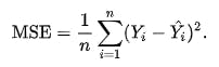
At first it might look intimidating, but I'm going to explain the symbols so that you can start to understand the notation for formulas like this one.

n stands for the number of instances (so if there are 10 instances - i.e. 10 violins, n=10)
The huge sigma (looks like a funky E) stands for "sum"
1/n is another way of writing "divide by the number of instances", since multiplying by 1/n is the same as dividing by n
Taken together, this part of the formula just stands for "mean" (i.e. average):
Then Y stands for the observed values of y for all the instances
And Ŷ (pronounced Y-hat) stands for the predicted y values for all the instances
Taken together, this part of the formula just stands for "square of the errors":
What do I mean by all the instances? That's if you made predictions on more than one violin at a time, and put all of those predictions into a matrix

The code: In the example below

X stands for all the instances of x - the features matrix
Y stands for all the instances of y - the ground truth labels matrix
w and b stand for the same things they did before: weight and bias

# import the Python library used for scientific computing 
import numpy as np 

# last week's predict function 
def predict(X, w, b):
    return X * w + b

def mse(X, Y, w, b):
    return np.average(Y - (predict(X, w, b)) ** 2)

At this point we know how wrong we are, but we don't know how to get less wrong. That's why we need to use an optimization function.

Optimizing predictions with Gradient Descent

This is the part of the process where the model "learns" something. Optimization describes the process of gradually getting closer and closer to the ground truth labels, to make our model more accurate. Based on the error, update the weights and bias a tiny bit in the direction of less error. In other words, you are making the predictions a little bit more correct. Then you check your loss again, and rinse and repeat until you decide you have minimized the error enough, or you run out of time to train your model - whichever comes first.

Now, I know I said I would discuss gradient descent this week, but I am starting to feel that doing it justice probably requires a whole post. Either this week's post will get too long, or I won't be able to unpack the details of gradient descent to a simple enough level. So, please bear with me and stay tuned for next week's Machine Learning Log, in which I will (promise!) discuss gradient descent in detail.

Madeline's Machine Learning Log